As teachers, we need to utilize data constantly. Google Forms is an excellent way to collect data from formative assessments. The purpose of formative assessment is to utilize the data to form what your next steps are. To reteach, to examine the quality of your instruction, to differentiate, to identify struggling students, etc…
Sorting the data in your spreadsheet helps you to quickly be responsive to your formative assessments. Try some of these techniques to help you sort in Google Sheets.
Sort Range
If you want to sort your data by class period, then by last name and then by first name that requires doing a multiple column sort.
If you have column headers you may want to freeze the first row. If you are using data from a Google Form the first row is already frozen for you.
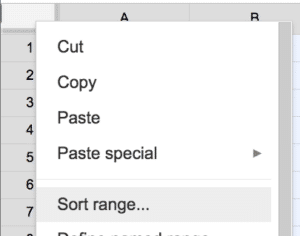
To the right of column A and above row 1 is a blank box. I will call this the “awesome box.” Clicking on the awesome box will select all cells in the spreadsheet. RIGHT CLICKING on the awesome box gives you options for the entire sheet.
Choose “Sort range…” from the right click options.
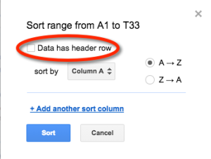
Check the checkbox that says “Data has header row”
Choose the initial column you want to sort by. Then click on “Add another sort column.”
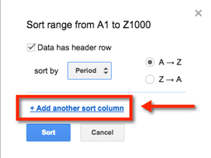
Repeat until you have selected all of the columns you want to sort by. Click the blue “Sort” button to sort the sheet.
Filter Icon
In the toolbar is an icon that looks like a funnel. Clicking this icon will turn on filter options for the entire sheet. If you want to only filter a particular range, highlight the range first. You may need to click on the “awesome box” or highlight a column before selecting the filter icon.
![]()
In the column headers or in the upper right of your selected range, drop down arrows will appear. This is NOT the same as the drop down arrow on the column indicators. The filter arrows will appear on the actual cells.

Clicking the drop down arrow shows a list of all of the values in the range of that column. By default all of the options are selected. To view rows that only show certain data values, click on “Clear” to uncheck all of the values.
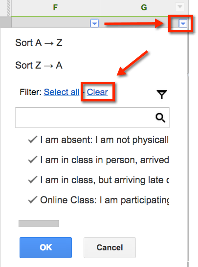
Click on the data values that you want to filter by. You can select multiple options. You can also use the search box in the filter options to help you locate the desired data more quickly. Click the blue “OK” button.
The rows of data that do not satisfy the filter are hidden. You can go back to the filter drop down arrows to change the filtering options.
Click on the filter icon in the toolbar to toggle off the filters. This will return the spreadsheet back to showing all of the rows of data.
![]()
Sort Sheet
Hover your mouse over the column indicators to reveal a drop down arrow.

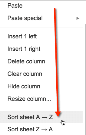
Clicking on this drop down arrow gives you a variety of options, one of which is to “Sort sheet A-Z.” This will sort the entire sheet by that particular column.
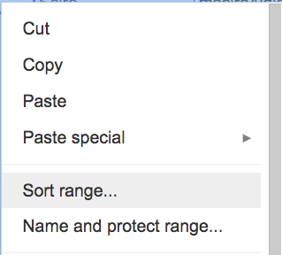
If you want to only sort a particular range on the spreadsheet and not the entire sheet, highlight the desired data. Right click and choose “Sort range.”
=SORT ( )
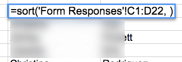
I usually prefer not to mess with my original data. I prefer to manipulate my Google Forms data in a separate tab. You can use the formula =sort( ) to bring data from one area of the spreadsheet to another.
=sort(range,column,true)
In a blank cell type =sort(
Highlight or type in the range of data that you want to have sorted.
Instead of saying the name of the column, you want to count how may columns you are sorting. If are possibly displaying multiple columns from your data but do not necessarily want to sort by the first column. After the comma put a 1 to sort by the first column, a 2 to sort by the 2nd column, a 3 to sort by the 3rd column, etc…
You will need another comma and to indicate “true” or “false” after the comma. True will sort the range by the indicated column from A-Z. False will sort Z-A.
![]()
If you have column headers do not include these in the sorting range. Your column headers will become sorted into the data.






1 thought on “4 Tips for Sorting in Google Sheets”
Wow, that =SORT() is soooooooooooo cooooooool because on top of filtering however I want, I’m also able to apply filters on it.
Thanks for sharing!!!