


When using a Google Spreadsheet you will likely want to freeze the first row and maybe the first few columns. What this does for you is allows you to see the header row as you scroll down through the spreadsheet. If you are looking at student data it is likely you would want to freeze the students name so that when you scroll to the right in the spreadsheet you are able to clearly connect the data to the students name.
By default the first row is frozen in the spreadsheet of a Google Form.
Upper Left
Look in the upper left hand corner of the spreadsheet. The square to the left of the column indicators and above the row indicators. I incorrectly refer to this as the “awesome box.” If you click on it, you select all of the cells in the sheet.
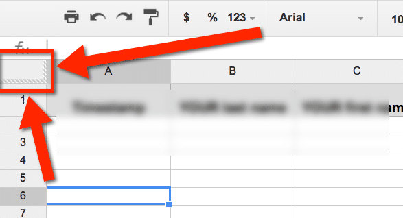
On the edge of the “awesome box” are hatched lines. These are the freeze bars.
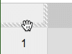
Grabby Hand
Hover your mouse over the edge of the “awesome box.” The cursor should change into a “grabby hand.”

Hold down your mouse and drag the freeze bar down. You can freeze multiple rows. You can also use the “grabby hand” to drag the vertical freeze bar to the right.
Once the freeze bars have been moved, you can use the “grabby hand” to move the freeze bars back if you need to. Note that sometimes in order to delete rows or columns or do other functions you need to return the freeze bars to their “resting” position back at the “awesome box”