Many to One

This school year I am trying to do my grading with a pivot table.  I am using mail merge to send students individualized feedback and their grade. What I haven’t quite been able to get nailed down is how to give students a list of their assignments in a paperless way. I could import the spreadsheet to a database and easily create reports per kid… but I’m trying to stay in Google.  I saw a plea go out on a list serve the other day for wanting to merge multiple rows to one row and I got a phone call the next day of someone asking me the same thing. So clearly I am not the only one in need of this ability.  Searching for scripts or on Google for solutions came up empty.  Ended up resorting to a complicated formula. So here is what I did… probably not for the faint of heart.  If you’re not fairly proficient with a spreadsheet I wouldn’t attempt it.  Try this blog post on pre-populating a Google Form instead.

First I have students fill out a Google Form that is embedded in my website to turn in all assignments.  (Sample form is embedded at the bottom, feel free to fill it out).

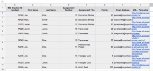
Here is link to my sample spreadsheet: http://goo.gl/YBCvS

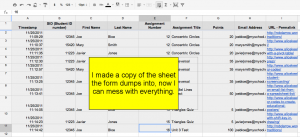
1. Make a copy of the sheet you’re working with. You don’t want to ruin your data accidentally.
2. Click on the upper left hand corner, right click and choose copy.  Right click again and choose paste special->paste values only.
3. Sort the spreadsheet by the column with the unique identifier (so that all of the rows you want merged together are grouped together.)
4. Insert a row for concatenation.  I can not actually merge all the rows together, so I need to get all the data from the single row into one cell.  I did =”#”&E2&” “&F2&” earned “&G2&” points”
   
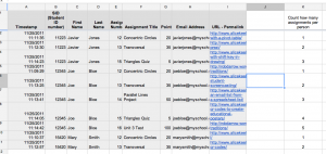
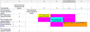
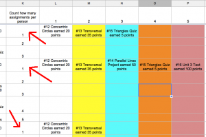
5. Create a column to number the entries. In column K I did =if(C2=C1,K1+1,1)
6. I used =max(K2:K300) to find out the most anyone had submitted the form.
7. I created a column for each of these submissions.  So since I had a max of 16, I created 16 extra columns.
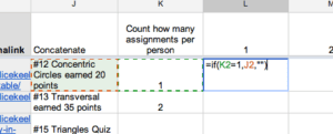
8. For the column that would contain the information from the first row, that is easy, I just said it equals what is in my concatenation column (J). =if(K2=1,J2,””)
9. Not everyone has a row 2 so I need to check if they do and then get the information from row 2’s concatenation cell. I did =if($B3=$B2,if($K3=M$1,$J3,””),””)
   I am checking if the unique identifier for the rows are identical.
10. Unfortunately you have to build each formula for each column almost by scratch.  I did a little cheating with that, but could not get away from editing each cell individually at least a little bit. Next row and column would be =if($B4=$B3,if($K4=N$1,$J4,””),””) and the next column =if($B5=$B4,if($K5=O$1,$J5,””),””)
11. If you did it correctly it is always checking one row below the first unique row for a person, 2 rows below the first row for that person, 3 rows below the first row for that person, etc… and putting in the one cell that contains all the information for that row.
12. Repeat until you have a column up to the maximum number of rows any person has.
13. You will now drag each diagonal corner up to the first row. (Moving the formula).
14. Click on the upper left hand corner, right click and choose copy.  Right click again and choose paste special->paste values only.
    This will allow you to now sort your data without messing up your formulas.
15. Sort by the row (K) which counted rows per person, you only need the row 1’s now.
16. Delete all the extra rows.
17. Can now run a mail merge with this merged data.

Sample Form: