In my Intro to Google Sheets spreadsheets webinar I showed 6 key skills that you need for teaching with Google Sheets spreadsheets. One of the things we covered in the webinar is how to create a seating chart using Google Sheets.
Resize the Cells
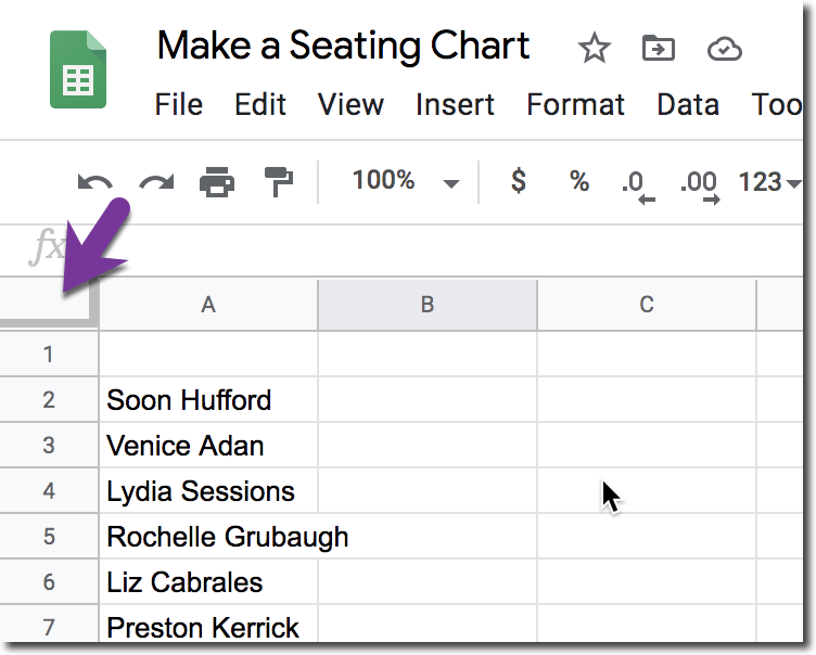
To the left of the column indicator A and above the row indicator 1 is the Awesome Box. This is a blank box in the upper left hand corner that when you click on it will select all.

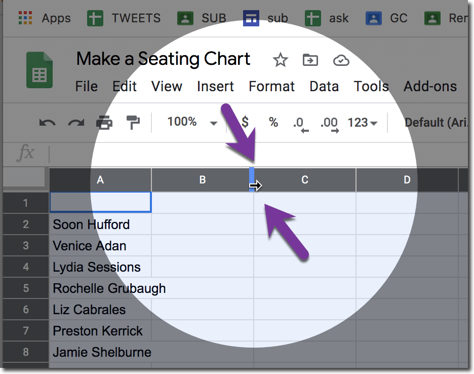
Now you can resize a column and resize a row and the entire spreadsheet will adjust. The idea is to make the cells of the spreadsheet resemble desks.

Randomize the Student Names
Highlight the student names and right click to choose “Randomize range.” This will help you create a random seating chart.

Drag Student Names
Single click on a cell with a student name. Get your mouse over the edge of the cell so that it turns into a gloved hand. Hold down with the mouse to have the hand grab the cell. Now drag the student name to where you want on the seating chart.
Format Your Seating Chart
Click again on the awesome box to select all. Find the centering icon in the toolbar to center the student names. The icon to the right of that allows you to center vertically. The icon to the right of that allows you to word wrap. This helps you get all of the student names shown in the cell.
Try using the paint can to color code your student groups.
Sample Spreadsheet
Here is a sample spreadsheet for you to try out making a seating chart. Notice the tabs along the bottom of the spreadsheet. Each step is laid out separately. Try creating your own seating chart!


3 thoughts on “Begin with Google Sheets: Make a Seating Chart”
The link for the Copy of Sample Spreadsheet takes me back to this page.
Thanks for the heads up. I updated it. Is this the one you needed? https://docs.google.com/spreadsheets/d/11LC9Wznt-fAV8_RtlrIoMPfu9euh03Yp4Gv6TGFFRgY/copy