I like to have my students conduct peer evaluations. The advantages are that students can receive some form of feedback faster than I can give feedback to everyone. Students are able to see work samples from other students to give them ideas of ways they could improve. They do their peer evaluations against the rubric with specific guided questions to help them give good feedback which helps the reviewer to better understand the requirements and to provide quality feedback.
I use Google Forms to accomplish this. The problem is how to send out the feedback back to the students. If 30 students evaluated the other students in the class that is roughly 900 emails to send out. Copying and pasting each one is not an option.
Note that Gmail now has a limit of 100 emails a day, it use to be 500. If you are using a GAfE account, that limit is 1500. Hopefully your school is on Google Apps. Sometimes I can max that out if I am sending out feedback from all 5 sections of my class. In those cases I share the spreadsheet with other Google accounts that I have and I send it partially from those.
If you are using the NEW Google spreadsheets the scripts are no longer working. You now must use the Add-Ons. Luckily there is a mail merge script for the new Google Sheets.
Note: It is important when you want to do a mail merge that you have the email addresses of the students you want to send the emails to.
Step 1: Create a Google Form
Create your Google Form that your students will fill out. Make sure the data from this Form goes into a spreadsheet. I have my settings to automatically create a spreadsheet each time I create a Google Form.
Step 2: Duplicate the Data
I cringe at the idea of destroying data. Most likely I will need to clean up the data a little bit. On the spreadsheet tab duplicate the Form Responses tab. Double click on the duplicated tab and rename it. I usually name this “Data.”
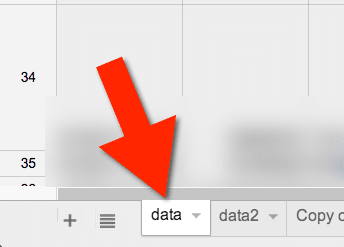
Step 3: Move the Data Tab to the First Position
You can click and hold down the mouse button on a tab to drag the tabs around. You want to move this tab to be in the first position.
Step 4: Create a New Tab
I need to do a little manipulation, thus I need some blank space to work. Click on the plus icon at the bottom left next to the tabs to create a new tab.
Step 5: Copy the First Row
The first row in your data spreadsheet contains the questions you asked. Probably you want to connect the information in the peer evaluation with the questions that were asked. Highlight the first row and copy it.
Paste this into the new tab you created.
Step 6: Transpose
In a cell below where you pasted the questions, use the formula =transpose( .
This will switch the questions from horizontal to vertical.
Step 7: Paste Special
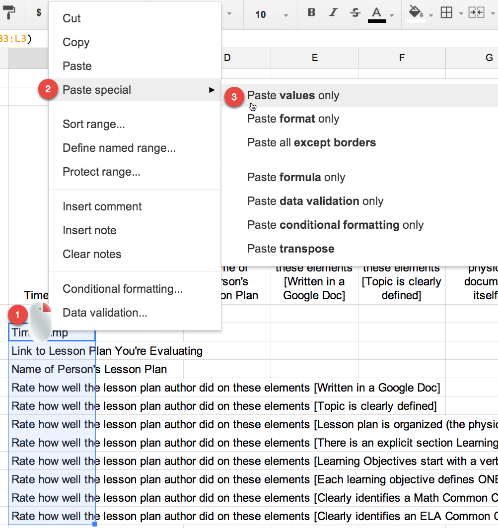
Now that your questions are vertical you will want to highlight them and right click. Choose paste special from the menu items and paste the values. This strips the transpose formula and leaves you with just the text.
Step 8: Shorten Titles
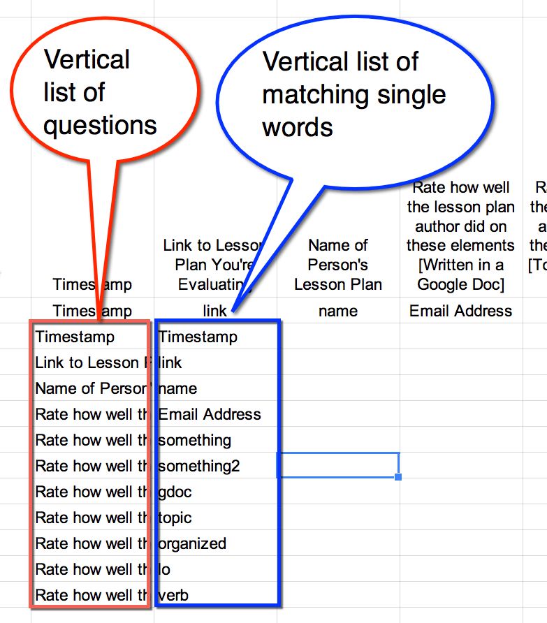
It is easier to manage a mail merge if your column headers are a single word. On the data tab replace each column header. You can not duplicate the column headers, make sure they are unique.
Step 9: Copy and Transpose
You need to pair up your original questions with your single word. After you have renamed the column headers on the data tab, copy those values. Paste them on the spreadsheet where you transposed your questions.
In the column next to the vertical questions you will want to transpose the list of single words. Use =transpose( again.
You will also want to highlight this transposed list, copy, right click, paste special.
Step 10: Add << >>
In the next column you will want to copy the question list again. You can avoid this step by putting the short words to the left of the questions to begin with. I like having them in this order though.
In the next column you are going to want to append << and >> to the front and end of the single words. These are the merge tags for the “Yet Another Mail Merge” Add-On.
=”<<“&C5&”>>
Obviously you want to replace the C5 with the location of the cell that has your first single word column header.
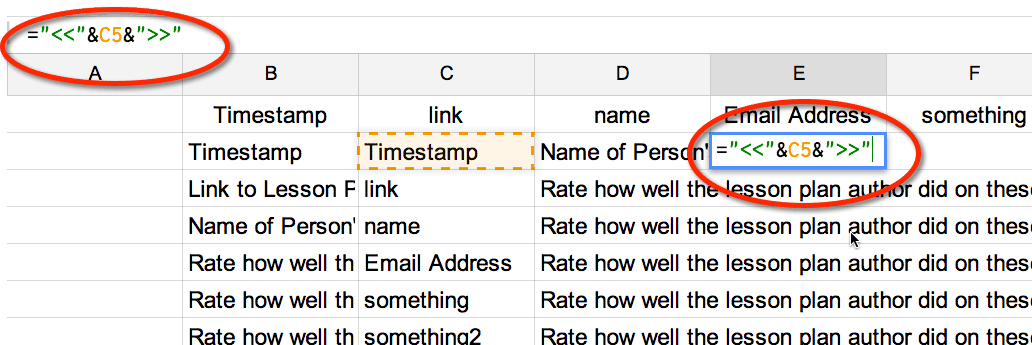
Copy and paste this formula for each single word column header.
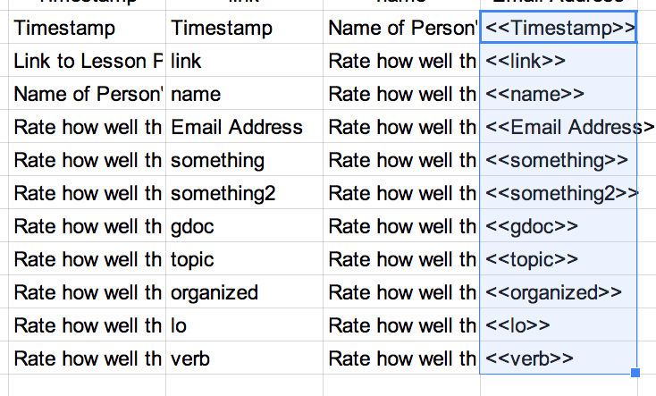
DELETE THE ROWS YOU DO NOT WANT TO SHARE WITH THE STUDENTS!
Some of the rows contain sensitive information such as the name and email of the reviewer. Some of the rows are data for me only.
Step 11: Craft an Email
Start a new email (Must be Gmail or GAfE email). You can use a merge tag anywhere you want to replace default text with what is in the spreadsheet. For example, I will have one column header titled “name.”
The merge tag is <<name>>. You must flank the column header with << and >> in order for the mail merge to replace.
For my subject line I will typically do something like
<<name>>, your peer feedback from your project
Somewhere in my email I will paste the two columns from the spreadsheet. Hint to widen the columns widths in the spreadsheet BEFORE you copy/paste.
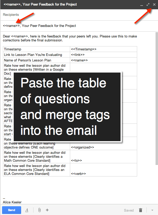
Step 12: X Out
You need to create a draft of the email. You do not send it to any recipients. Gmail saves your email automatically. You can close out of the email. It will be saved in drafts.
Step 13: Add-On
Back in the spreadsheet make sure you are on the data tab.
Add the Add-On “Yet Another Mail Merge.”
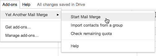
At the top is a menu option for “Add-ons.” Choose to “Get add-ons…” and type “mail merge” into the search. Install the “Yet Another Mail Merge.”
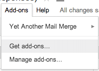
Go back to the Add-ons and choose to start the mail merge.
Step 14: Choose Draft and Send
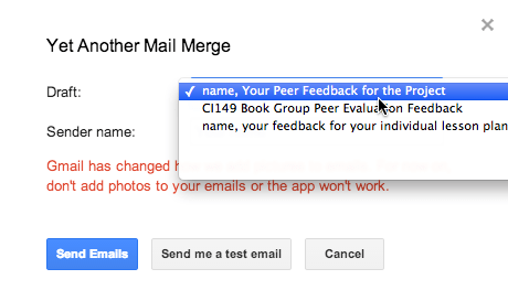
The first option is looking at your drafts. Find the draft email subject line that you want to send. For “Sender name:” you can type in who you want it to look like the email to come from. Usually I type my name, sometimes I get more creative. Click the blue button to “Send Emails.”
