Find Unique Data in a Spreadsheet
A function unique to Google Sheets is =UNIQUE(). This can be really handy when you have data from say a Google Form that repeats information and you want to find out how many unique instances there are. For example what if you use a Google Form to have students check out reading books or to sign out for the bathroom. The same student will fill out the form more than once. So you have a long list of student names, who actually went to the bathroom this semester? You need a list of the unique names with no repeats.
Sample Spreadsheet
I created a spreadsheet with a list of names that have repeating values. There are 632 names in the list. Have fun tallying by hand whose on the list minus repeats. Clearly that is crazy, this is where spreadsheets come to the rescue.
=UNIQUE()
In any blank cell type =UNIQUE( and then highlight the range of data with the list of values. For my sample spreadsheet it would be =UNIQUE(C2:C633). Press enter.
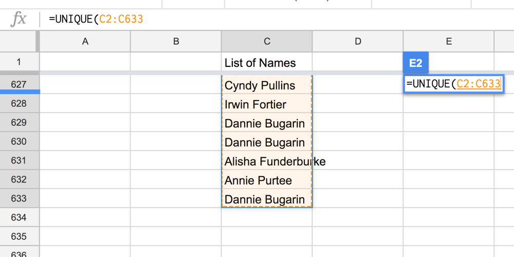
Rather than highlighting an entire column of data, you can use C:C to indicate a range of column C. In the case of this sample data range we do not actually want to include C1 since it is the column header and not a data value. So you can use the range C2:C to indicate start at row 2 and keep going for the rest of the column.

Shorter List
And so it turns out there are only 20 unique values out of the list of 632 names.

Pivot Table
The =UNIQUE() was helpful, but you might also want to know how many times each of these students went to the bathroom. This is where a Pivot Table comes in. Google just updated Pivot Tables for Google Sheets, it’s pretty exciting! For the sample spreadsheet click on column C to highlight the entire column. Go to the Data menu and choose “Pivot table.” Google is apparently also really excited about the new Pivot Table since the menu has a flag indicating “Updated.” I’ve never seen that before.
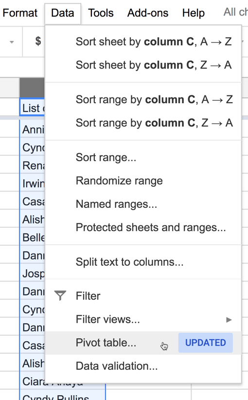
What a Pivot Table is good for is summarizing data that repeats! (It does other things too, but let’s just start with that.)
Pivot Table Editor
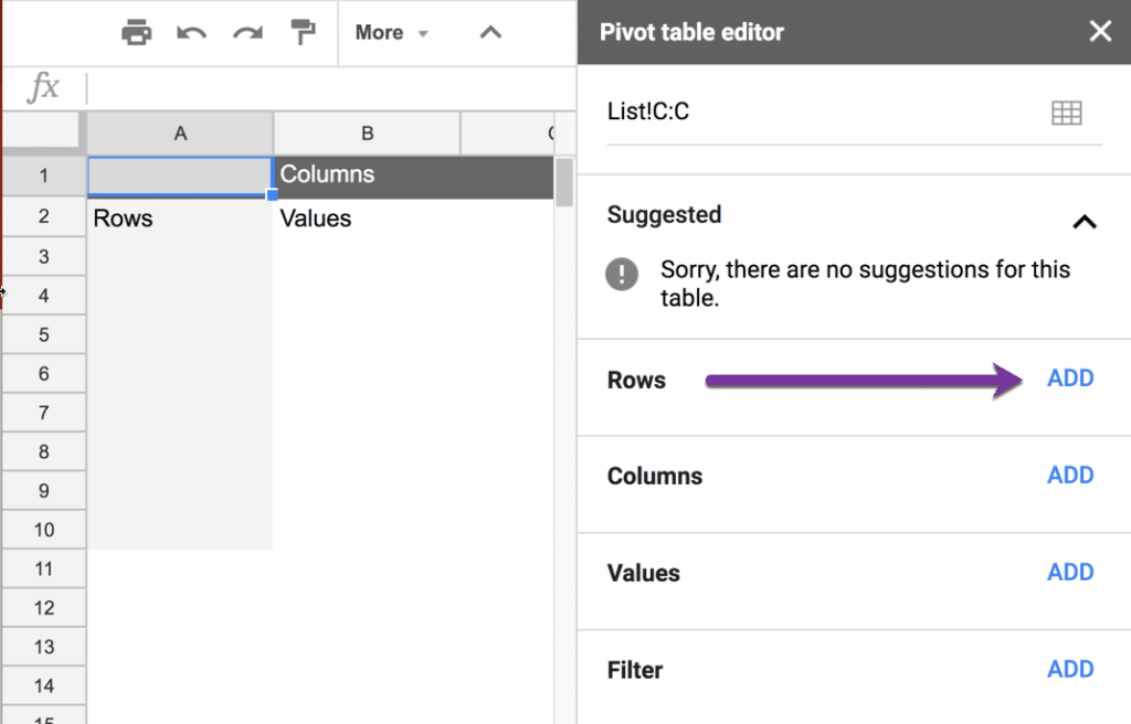
The new Pivot Table Editor will attempt to guess what kind of Pivot Table you want based on your data and give you suggestions. Unfortunately for this sample data, it has no clue.
Add Rows
Click on the Add button for Rows to choose the column of data that you want to summarize. Lucky us, there is only one column in this data set.
Values
Now, what values do you want to summarize? In this case, again we only have one column of data so that makes it easy.

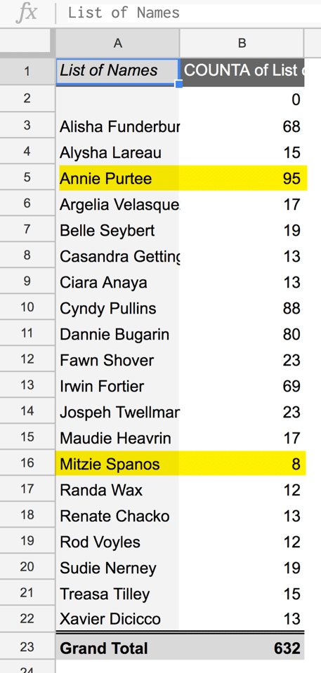
The new Pivot Table Editor is smart enough to look at what type of data you have and suggest how you might want to summarize the data. No more defaulting to SUM. Notice the pivot table suggests summarizing by “COUNTA.” This is probably the option I choose most often. The A stands for Alpha. It is counting alphanumeric values. COUNT only counts numbers.
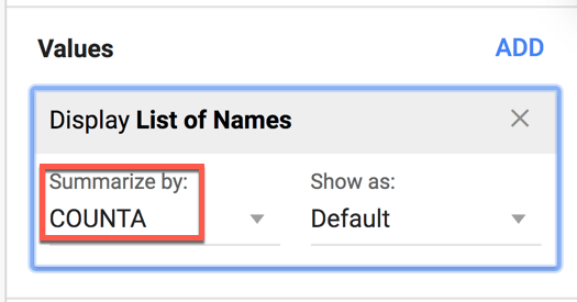
Since our list is not a list of numbers then COUNTA is the best choice for counting how many times each name shows up. Like magic, the pivot table shows me that Annie went to the bathroom 95 times! Whoa!


1 thought on “Google Sheets: =UNIQUE()”
Exactly what I needed. Thanks 🙂