$A$5
Cell referencing is when you use a formula to refer to a cell. In a spreadsheet you start a formula with an equals sign (=) and then command the spreadsheet to complete a task.
Example: typing =5+6 into a cell and pressing enter will calculate the value and return 11.

Cell Referencing
The problem with typing formulas like this is what happens if one of those values changes? You must then double click on the cell containing the formula and edit the number. This is particularly problematic if you are using that same value in multiple cells.
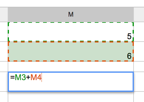
As much as possible I try not to enter values into a formula. Instead I refer to a cell that contains that value. Somewhere on the spreadsheet I will type my values into a cell. The cell that I want to have the calculated value I will start with an equals sign and then type in the reference to the cell or click on the cell to have the spreadsheet automatically populate the value. For example if I typed a 5 into cell M3 and 6 into cell M4 then my formula would be =M3+M4 instead of =5+6. This means if I change the value in cell M3 the sum of the two numbers will automatically update.

Notice that by CLICKING on a cell the cell reference is automatically inserted for you.
This is particularly useful as a teacher when you are calculating rubric scores or adding up a students points. I use Google Forms to collect all sorts of data from my students. I am able to send these results to a spreadsheet. Using cell referencing makes it easy for grading, calculating and other tasks.
Absolute Cell Referencing
Oftentimes you will find that you are using the same number repeatedly in calculations. One example is in calculating a students score you divide each students score by the number of points possible. This number of points possible remains constant for all students in the class.
When you fill down in a spreadsheet it copies the pattern. So if I tell the spreadsheet to take the number to the left of a cell and divide it by the number above the cell, if I fill down (copy) the formula it actually copies the pattern.
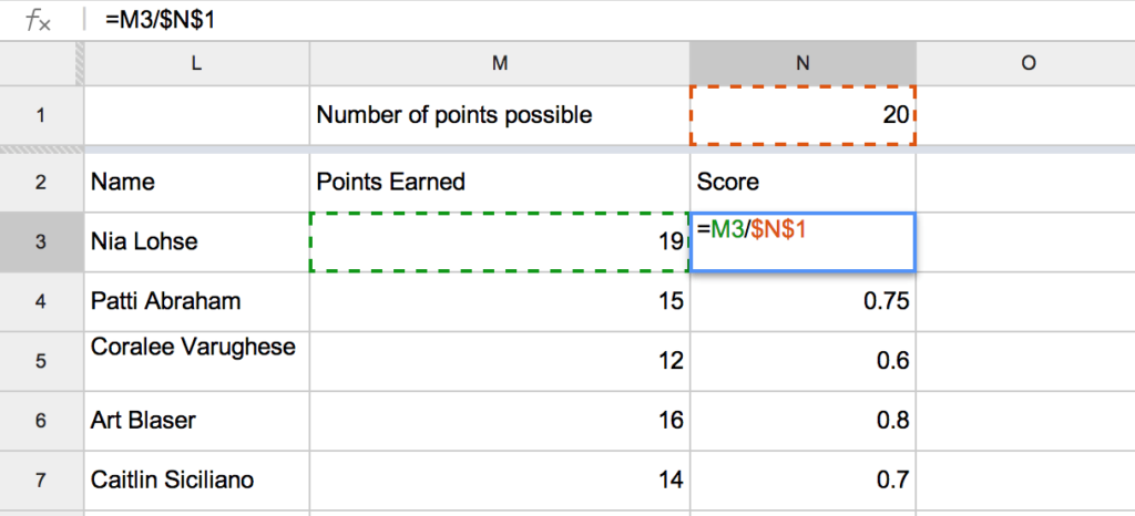
Create a cell for the number of points possible for an assignment. Looking at a roster of students with their quiz score next to their name you will want to calculate their percentage. In the cell next to a students name you enter the formula =(points earned)/(points possible). For each student the number of points they earn is in a different cell, but the points possible cell remains the same so you will want to freeze that cell.

Notice in the screenshot above Nia’s grade is calculated with the formula =M3/$N$1.
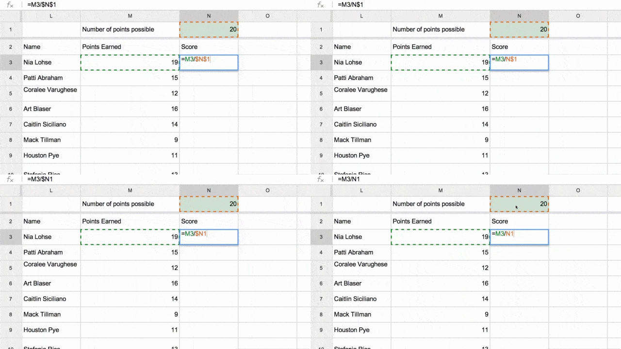
The key to absolute cell referencing are those DOLLAR SIGNS in the formula.
The dollar sign in front of the N locks down column N. The dollar sign in front of the 1 locks down row one.
$$
Type a dollar sign ($) in front of the Letter and/or Number of the spreadsheet cell to absolutely reference that particular cell even if you copy and paste the formula.
$C$5
$C$5 locks down cell C5.
$C5 only locks down column C, but would allow for $C6, $C7, $C8, etc… when copying and pasting the formula.
C$5 only locks down row 5, but would allow for D$5, E$5, F$5, etc… when copying and pasting the formula.
Keyboard Shortcut – F4
It can be cumbersome to type the dollar signs into your formulas in a Google Spreadsheet. When typing your formula, immediately after clicking on a cell to select it for your formula select the F4 key. Striking the F4 key once will create double dollar signs on that cell reference. It will NOT create double dollar signs on all of the cell references in the formula. Strike the F4 key again and the dollar sign is only on the row. Strike the F4 key a 3rd time to toggle to the dollar sign only being on the column. A 4th strike of the F4 key will return the cell reference to normal, no dollar signs.


5 thoughts on “Google Spreadsheets: Absolute Cell Referencing”
Thanks! It was really helpfull
Hi
We are doing a similar thing
Person fills out google form
Contents goes into ‘Spreadsheet 1’
In Spreadsheet 2, it uses some data to display from entries in Spreadsheet 1.
In Spreadsheet 2
We have in a cell =’Spreadsheet 1’A3 (or =’Spreadsheet 1’$A$3)
So say someone adds a form Entry with the text Chicken, so the text ‘Chicken’ appears in Spreadsheet 1, cell A3
However the form goes and updates what I had in Spreadsheet 2 to be =’Spreadsheet 1’A4 which is obviously blank.
It seems like adding a new line on the original spreadsheet (via a form) causes the form to force the cell formula to update, even if you use $’s to make it absolute.
Can this be turned off?
Thanks
The form responses tab is not going to behave like “normal” tabs since it is dynamic in taking data from the Google Form. I use =importrange to help solve this issue that when you reference the form responses tab and new data is added that your formulas on other tabs do not update. So use =importrange on a different tab that brings in the data from Form Responses and then write your formulas to reference the new tab.
On a chromebook without function keys, use SEARCH+4 or SEARCH+FULLSCREEN to use the function key F4. You can see all possible keyboard shortcuts with CTRL+ALT+SHIFT+?, then hit the search (magnifying glass) key to see all the function key mapping.
I’m having the same issue as Tom G but I can not import with rest of my formula. Here is my current formula that is in a different tab called POST. =RIGHT(Pull!$A$1381,LEN(Pull!$A$1381)-FIND(“=”,Pull!$A$1381)) but like Tom said when data is posted into the PULL tab the the numbers change in the POST tab even know they are locked.